Welcome to BioPredict

A pilot app modelling and predicting biodiversity on Irish Sea coastal structures


Artificial structures are built along coastlines globally to protect property but also provide access for sea-based activities. There is growing interest in being able to predict the biological communities that will colonise new structures, given their potential to provide stepping-stones for problem species and/or to provide surrogate habitats for coastal biodiversity.

This pilot app uses new and existing data describing the physical features (e.g. material, structure type); environmental context (e.g. wave exposure, salinity) and biological communities of 69 intertidal artificial structures around the Irish Sea coasts of Wales and Ireland. It can be used to model the relationships between the physical and environmental parameters (‘predictor variables’) and a range of biodiversity metrics calculated for each structure.

The tool provides four different ways of exploring the data and the models, as indicated in the boxes below. Each can be accessed via the tabs above.


Additional project outputs and resources

Ecostructure has undertaken numerous and comprehensive assessments of the Irish Sea area in regard to community composition, functional valuations and site connectivity. We are keen to offer users links to the other important outputs .


1. Metadata and GIS maps of artificial structures along the Irish (Counties Louth - Cork) and Welsh coastlines.

This data formed part of mapping work including observations of intrinsic (size, length, type of structure, material) and extrinsic features of the artificial structures, as published in Thompson, Crowe & Brooks (2021) Ocean & Coastal Management.


2. The following link provides access to data gathered via remote sensing techniques namely LiDAR and UAV obtained from a selection of artificial and natural study sites along the Irish and Welsh coastlines.


3. Ecosystem functions are vital for understanding the roles and value of species within a given location. Here, you can find a tool (including a refence guide and case studies) and resulting predictive model to explore how different communities can lead to different provisions of these important ecosystem functions.


4. Finally Ecostructure also aimed to review the likely dispersal of particles/larvae to highlight connectivity between locations and thus possible 'sink' locations for potentially invasive species can be found here. Please seek contact with a member of the Ecostructure team for login credentials.


Please note: the data provided in all links above still subject to publication by members of the Ecostructure project team. If you intend to publish any data, in part or full, and/or if you are having difficulty accessing the data, please contact the Ecostructure team.


Code and data are archived below:

DOI

Biodiversity on the Irish Sea coastal structures - map the data

This page allows you to map the data used to build this Ecostructure tool. You can view the survey sites (69 artificial coastal structures) arounds the Irish Sea and see what biodiversity was recorded on them. Step 1 allows you to choose the type of data to view - abundance scores for predefined groups, or biodiversity index scores (species richness, functional richness). Steps 2 and 3 allow you to filter by structure features and/or site context.

Please note in the top right there is the option to reset inputs back to default.

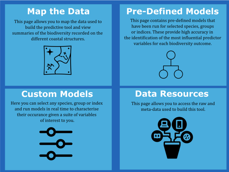
Step 1: Choose data to map

The left-hand drop-down menu allows you to view a selection of pre-defined species groups or overall biodiversity index scores.

Alteratively, select 'Custom Species' at the bottom of the left-hand drop-down box to activate the righ-hand menu and create your own species groups or singular species selections.


Step 2 (optional): Filter by material, structure type and urban/rural setting.

Default, all sites selected. Choose data to view by de-selecting options from the buttons below. Please refer to the 'Data Resources' tab for infomation regarding how variables were measured.


Step 3 (optional): Filter by environmental condition

Choose the data to view by selecting a variable from the drop-down menu, then either; all the sites (default), or those with values higher or lower than the median.


View your data selection on the map below

Data are represented by coloured symbols graduating from red (low) to green (high) within the range selected in step 1. Please click on the symbols to view the data for each site.


Pre-defined models of biota and biological indices

These pre-defined models have been run for selected species/groups/indices and provide the greatest level of accuracy in identifying the most influential predictor variables and characterising their influence and the uncertainty associated with the resultant model outputs.

The Custom Models tool on the next tab enables you to select any species, group or index and run models in real time, but the outputs are less reliable than those presented on this tab.

Step 1: Select a: Species / Group or Biological Index


Step 2: Explore the model outputs


1. Decision Tree

The branching white boxes in the tree show variables (environmental and/or context) required to best classify our sites in relation to a “pass” or “fail”

The end points (coloured red to green) are known as leaves. In each leaf the text indicates the most likely outcome (PASS or FAIL). The two numbers indicate the probabilities of the species or index being (a) below and (b) above the pass-fail threshold under the environmental conditions specified in the branches of the tree leading to that leaf.

The depth of colour of the leaves is representative of the confidence (and the volume of data falling with that leaf) in the prediction. Leaves that are bright green or bright red indicate confident predictions of pass or fail respectively (with a probability of 0.85 or greater). Pale green or orange colours indicate less confidence (or similar probinilties as above but less data). Yellow leaves represent classifications that should be considered with caution. These leaves have proportions closer to “.60 / .40“ or “.50 / .50“. Here the algorithm will still suggest the most likely outcome but the supporting evidence is not clear-cut.


2. Model Accuracy

Here we present the results of a simple accuracy assesemnt known as a confusion matrix.

Here we present the results of a simple accuracy assessment known as a confusion matrix. In this grid the perfect model would classify data into either the top left and top right boxes known as true positive (TP) and true negative (TN).

Classifications within the top right box indicate sites that PASS the threshold being predicted as FAIL. Classification in the bottom right corner indicate sites that FAIL the threshold being predicted to PASS.


3. How many variables best predict the chosen index?

In this line plot are the results of a further machine learning algorithm called recursive feature elimination (RFE). The computer attempts to use every combination of our variables and calculate the typical accuracy of models containing these many variables.

The dots at each point along the x-axis represent the average performance for models containing that many variables. We as a result want to create models with as high score as possible but also as simple as possible so look for a clear plateau and use this construction for our final predictions.


4. What are the best variables to predict the chosen index?

There are several ways of identifying the “best” variables from a list of candidates. The method used here is a further product of the machine learning algorithm used above. Here the variables are scored in terms of 1) their importance and, 2) their occurrence in the computer runs.

The y- axis, presents the loss of predictive skill when leaving that variable out. A high score meaning the model is worse without this variable.

The x-axis shows the average depth or stage the computer requires this variable within its decision trees. The lower the number the more readily required the variable.

Typically, variables plotting towards the top left are the most valuable. All the variables within the plot are important to some degree, however those with dots outlined in black are the ”best of the best”.

Custom models of biota and biological indices

This 'Custom Models' tool enables you to select any species, group or index and run models in real time to characterise their occurence according to the predictor variables, but the outputs are less reliable than those presented on the 'Pre-defined Models' tab.

1. Choose variables

Abundance Data:

Presence / Absence Data:

Select predictor

2. Explore and select threshold

Select a threshold

This setting enables you to specify the level of abundance or richness above which the model indicates an occurrence of the selected species/group.

Values and Threshold

3. View Model

Model Tree

Data resources

On this page we provide meta-data and infomation regarding data sources used in the production of this Ecostructure output.

Resource 1: Ecostructure Data

Please click on the resources below (2&3) to download the environmental and biological meta-data.

Please be sure to acknowledge the data source of this tool if used in publications or other applications. Recommended citation available at:

DOI

Working title: Lawrence P.J., et al “Predicting biological communities on artificial coastal structures“

Ecostructure would like to recognise all the key partners:

Paul Brooks, Jennifer Coughlan, Veronica Farrugia Drakard, Donal Lennon, Bryan Thompson & Tasman Crowe (University College Dublin)

Peter Lawrence, Tim D'Urban Jackson, Stuart Jenkins, Liz Morris-Webb, Siobhan Vye & Andy Davies* (Bangor University (* & University of Rhode Island))

Ally Evans, Hannah Earp, Liz Humphreys, Tomos Jones, Melanie Prentice, Harry Thatcher & Pippa Moore* (Aberystwyth University (* & Newcastle University))

Tom Fairchild & John Griffin (Swansea University)

Amy Dozier & Kathrin Kopke (University College Cork)

Further thanks to Keaton Wilson (University of Arizona) and Paula Gutiérrez-Muñoz (Instituto de Investigaciones Marinas (CSIC))

Special thanks to the steering committee for guidance and feedback. We further acknowledge the early roles that Dr. Louise Firth and Prof. Steve Hawkins played with Ecostructure colleagues in identifying the need for and developing the concept of such tools

Resource 2: Meta-data (Environmental variables).

Please click on the tab below to download the environmental meta-data.


Resource 3: Meta-data (Biotic data collection).

Please click on the tab below to download the biotic meta-data.